Guide to Adstock Transformations in PyMC-Marketing#
This notebook provides a comprehensive overview of the different adstock transformations available in PyMC-Marketing. Adstock effects model the delayed and lagged impact of marketing spend on consumer behavior.
What is Adstock?#
Adstock (also called the carryover effect or lagged effect) is a fundamental concept in marketing that models how advertising impact doesn’t happen instantaneously. Instead, it builds up over time and gradually decays.
The Core Idea#
When you run an advertising campaign, the effects don’t just appear in the same week and then disappear completely. There are three major behaviors that we need to keep in mind:
Memory effect: Consumers remember your ad after seeing it (think of that jingle from a TV commercial you saw years ago)
Delayed response: It may take time for someone to act on your advertisement
Gradual decay: The impact slowly fades over subsequent time periods
Why Adstock Matters for MMMs#
Understanding adstock effects is crucial for:
Budget Planning: If a channel has long-lasting effects, you might advertise less frequently but still maintain impact
Attribution: Correctly assigning sales to the marketing that caused them, even if there’s a time lag
ROAS Calculation: Ensuring you capture the full return, not just immediate effects
Channel Comparison: Different channels have different decay patterns (e.g., TV ads vs. digital banner ads)
Mathematical Representation#
The simplest form is Geometric Adstock, where the transformed value at time \(t\) is:
Where:
\(x_t\) is the raw advertising spend at time \(t\)
\(\tilde{x}_t\) is the transformed (adstocked) value
\(\alpha \in [0, 1]\) is the retention rate (how much of the effect carries over)
Higher \(\alpha\) means slower decay (longer-lasting effects)
This creates an exponential decay pattern where the effect of advertising in week 0 continues into weeks 1, 2, 3, etc., diminishing by factor \(\alpha\) each period.
Types of Adstock in PyMC-Marketing#
The library offers several adstock transformations to model different decay patterns:
Geometric Adstock: Simple exponential decay (most common, good default choice)
Delayed Adstock: Adds a delay parameter, peak effect happens after \(\theta\) periods
Weibull PDF/CDF Adstock: More flexible decay curves that can model peak-then-decay patterns
Binomial Adstock: Alternative flexible decay specification
Real-World Intuition#
Different advertising channels exhibit different decay patterns:
Digital display ads: Might have \(\alpha \approx 0.2\) (fast decay, effects last 1-2 weeks)
TV brand campaigns: Might have \(\alpha \approx 0.7\) (slow decay, effects last months)
Billboard advertising: Might have delayed peak if it takes time for brand awareness to convert to action
The adstock transformation ensures that when you model sales as a function of marketing spend, you’re capturing the full temporal dynamics of how advertising actually influences consumer behavior.
The Layout#
This guide has the following sections:
Geometric Adstock — the workhorse, simplest and most widely used
Delayed Adstock — adds a delay/lag parameter
Weibull CDF Adstock — S-shaped curve, gradual build-up
Weibull PDF Adstock — peak effect, then decay
Binomial Adstock — flexible alternative parametrization
Comparison — visual comparison across all functions
Each section includes:
When to use it
Mathematical formulation
Parameter explanations
Visualizations with different parameter values
# Import required libraries
import matplotlib.pyplot as plt
import numpy as np
import pandas as pd
import plotly.graph_objects as go
import plotly.io as pio
import pytensor.xtensor as ptx
import seaborn as sns
from plotly.subplots import make_subplots

from pymc_marketing.mmm import (
    BinomialAdstock,
    DelayedAdstock,
    GeometricAdstock,
    WeibullCDFAdstock,
    WeibullPDFAdstock,
)
from pymc_marketing.mmm.transformers import (
    WeibullType,
    binomial_adstock,
    delayed_adstock,
    geometric_adstock,
    weibull_adstock,
)

pio.renderers.default = "notebook_connected"

# Set plotting style with colorblind-friendly palette
sns.set_style("whitegrid")
sns.set_palette("colorblind")
plt.rcParams["figure.figsize"] = (14, 6)
%config InlineBackend.figure_format = "retina"

# Define colorblind-friendly colors for consistent use
CB_COLORS = sns.color_palette("colorblind")
COLOR_CH1 = CB_COLORS[9]
COLOR_CH2 = CB_COLORS[2]

# Load the example dataset
url = "https://raw.githubusercontent.com/pymc-labs/pymc-marketing/main/data/mmm_example.csv"
data = pd.read_csv(url, parse_dates=["date_week"])
print(f"Dataset shape: {data.shape}")
data.head(10)
Dataset shape: (179, 8)
| date_week | y | x1 | x2 | event_1 | event_2 | dayofyear | t | |
|---|---|---|---|---|---|---|---|---|
| 0 | 2018-04-02 | 3984.662237 | 0.318580 | 0.000000 | 0.0 | 0.0 | 92 | 0 |
| 1 | 2018-04-09 | 3762.871794 | 0.112388 | 0.000000 | 0.0 | 0.0 | 99 | 1 |
| 2 | 2018-04-16 | 4466.967388 | 0.292400 | 0.000000 | 0.0 | 0.0 | 106 | 2 |
| 3 | 2018-04-23 | 3864.219373 | 0.071399 | 0.000000 | 0.0 | 0.0 | 113 | 3 |
| 4 | 2018-04-30 | 4441.625278 | 0.386745 | 0.000000 | 0.0 | 0.0 | 120 | 4 |
| 5 | 2018-05-07 | 3677.396550 | 0.047171 | 0.000000 | 0.0 | 0.0 | 127 | 5 |
| 6 | 2018-05-14 | 5067.546337 | 0.424249 | 0.000000 | 0.0 | 0.0 | 134 | 6 |
| 7 | 2018-05-21 | 6079.099042 | 0.333920 | 0.879782 | 0.0 | 0.0 | 141 | 7 |
| 8 | 2018-05-28 | 4954.205369 | 0.253070 | 0.000000 | 0.0 | 0.0 | 148 | 8 |
| 9 | 2018-06-04 | 5865.676576 | 0.938054 | 0.000000 | 0.0 | 0.0 | 155 | 9 |
def adstock_timeseries(x, func, **kwargs):
    """
    Apply adstock transformation to time series data.

    Parameters
    ----------
    x : array-like
        The input time series data (e.g., marketing spend values)
    func : callable
        The adstock function to apply (e.g., geometric_adstock, delayed_adstock, etc.)
    **kwargs
        Additional keyword arguments to pass to the adstock function.
        Common parameters include:
        - alpha: retention rate
        - theta: delay parameter (for delayed adstock)
        - lam, k: Weibull parameters
        - l_max: maximum lag periods
        - normalize: whether to normalize the decay curve
        - dim: dimension name (typically "time")

    Returns
    -------
    np.ndarray
        The adstock-transformed time series

    Examples
    --------
    >>> # Apply geometric adstock
    >>> x_geo = adstock_timeseries(
    ...     data["x1"].values,
    ...     geometric_adstock,
    ...     alpha=0.5,
    ...     l_max=12,
    ...     normalize=True,
    ...     dim="time",
    ... )

    >>> # Apply delayed adstock
    >>> x_delayed = adstock_timeseries(
    ...     data["x1"].values,
    ...     delayed_adstock,
    ...     alpha=0.6,
    ...     theta=2,
    ...     l_max=12,
    ...     normalize=True,
    ...     dim="time",
    ... )
    """
    return func(ptx.as_xtensor(x, dims=("time",)), **kwargs, dim="time").eval()
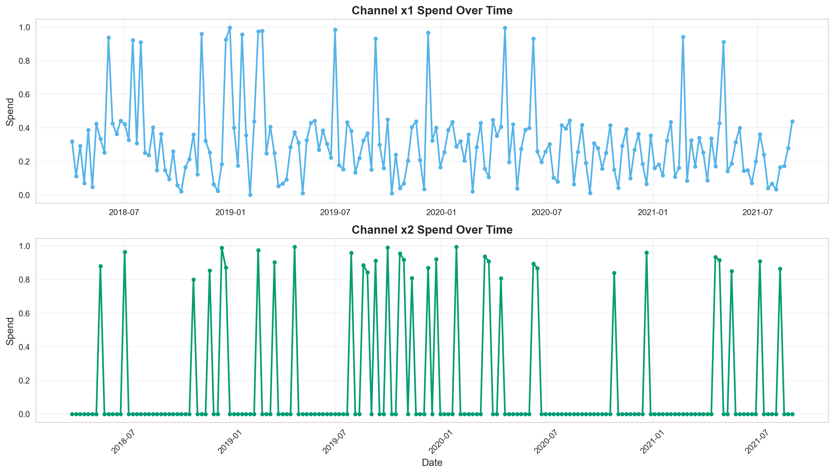
Understanding the Data#
Let’s visualize our marketing spend channels (x1 and x2) over time:
# Create subplots for the original time series of channels x1 and x2
fig, axes = plt.subplots(2, 1, figsize=(14, 8))

# Plot channel x1
axes[0].plot(
    data["date_week"],
    data["x1"],
    marker="o",
    linewidth=2,
    markersize=4,
    color=COLOR_CH1,
)
axes[0].set_title("Channel x1 Spend Over Time", fontsize=14, fontweight="bold")
axes[0].set_ylabel("Spend", fontsize=12)
axes[0].grid(True, alpha=0.3)

# Plot channel x2
axes[1].plot(
    data["date_week"],
    data["x2"],
    marker="o",
    linewidth=2,
    markersize=4,
    color=COLOR_CH2,
)
axes[1].set_title("Channel x2 Spend Over Time", fontsize=14, fontweight="bold")
axes[1].set_xlabel("Date", fontsize=12)
axes[1].set_ylabel("Spend", fontsize=12)
axes[1].grid(True, alpha=0.3)

plt.xticks(rotation=45)
plt.tight_layout()
1. Geometric Adstock#
Overview#
Geometric adstock is the simplest and most commonly used adstock transformation. It models a constant exponential decay where the effect diminishes by a fixed proportion each time period.
Mathematical Form#
Where:
\(x_t\) is the raw advertising spend at time \(t\)
\(\tilde{x}_t\) is the transformed (adstocked) value
\(\alpha \in [0, 1]\) is the retention rate (how much of the effect carries over)
Higher \(\alpha\) means slower decay (longer-lasting effects)
When to Use#
Default choice for most marketing mix modeling applications
When you expect a simple, consistent decay in advertising effect
Digital advertising (display ads, search ads) where effects typically fade uniformly
When you have limited data or want model simplicity
Awareness campaigns where impact gradually declines
Parameters#
alpha: Retention rate (0-1). Higher values = slower decayl_max: Maximum lag periods to consider
Generate Geometric Adstock Instance#
Here we create a Geometric Adstock instance to help explore different behaviors.
We instantiate the GeometricAdstock transformer with two key parameters:
l_max=12: Maximum lag to consider (12 weeks). This defines how far back in time the adstock effect extends. For weekly data, 12 weeks (~3 months) is common.normalize=True: Ensures the adstock weights sum to 1, making the transformation interpretable as a weighted average of past spend values.
Before fitting a model, it’s useful to visualize what the adstock transformation looks like under different parameter values:
sample_prior(): Generates random parameter values (alpha) from the prior distributionsample_curve(): Uses those parameters to create the actual decay curve
# This instance will be used to transform raw marketing spend data into adstocked
# spend that accounts for the carryover effects over time.
geometric = GeometricAdstock(l_max=12, normalize=True)

# Sample the prior and curve
# This helps us understand the range of decay patterns our model considers plausible
# BEFORE we see any data. It's a sanity check that our priors make sense.
rng = np.random.default_rng(42)
prior = geometric.sample_prior(random_seed=rng)
curve = geometric.sample_curve(prior)

print("Geometric Adstock Configuration:")
print(geometric)
Sampling: [adstock_alpha]
Sampling: []
Geometric Adstock Configuration:
GeometricAdstock(prefix='adstock', l_max=12, normalize=True, mode='After', priors={'alpha': Prior("Beta", alpha=1, beta=3)})
If you noticed when running the above cell, we print out the geometric object. This enables us to look into how we configured our Adstock effects. Let’s dive into the priors!
priors: A dictionary specifying the prior distribution for thealphaparameter (retention rate). For example,Prior("Beta", alpha=1, beta=3)creates a Beta(1,3) prior that favors lower alpha values (faster decay), which is often reasonable for marketing effects.
The alpha parameter (\(\alpha \in [0, 1]\)) controls the retention rate:
\(\alpha = 0\): No carryover effect (only immediate impact)
\(\alpha = 0.5\): Moderate decay (effect halves each period)
\(\alpha = 0.9\): Very slow decay (long-lasting memory effect)
Tip
We also allow you to choose when to transform the spend. Whether it’s before or after the saturation transformation. See below!
mode: Determines when the adstock transformation is applied in the model pipeline:'After': Apply adstock after saturation transformations (most common)'Before': Apply adstock before saturation transformations
Decay Curves for Different Alpha Values#
fig, ax = plt.subplots(figsize=(12, 6))

# Test different alpha values
alphas = [0.2, 0.4, 0.6, 0.8, 0.9]
l_max = 12

# Create impulse (single unit of spend at time 0)
impulse = np.zeros(l_max)
impulse[0] = 1.0

for alpha in alphas:
    result = geometric_adstock(
        ptx.as_xtensor(impulse, dims=("time",)),
        alpha=alpha,
        l_max=l_max,
        normalize=False,
        dim="time",
    )
    ax.plot(range(l_max), result.eval(), marker="o", linewidth=2, label=f"α={alpha}")

ax.set_xlabel("Time Periods Since Spend", fontsize=12)
ax.set_ylabel("Effect", fontsize=12)
ax.set_title(
    "Geometric Adstock: Decay Curves for Different α Values",
    fontsize=14,
    fontweight="bold",
)
ax.legend(fontsize=11)
ax.grid(True, alpha=0.3)
plt.tight_layout()
plt.show()
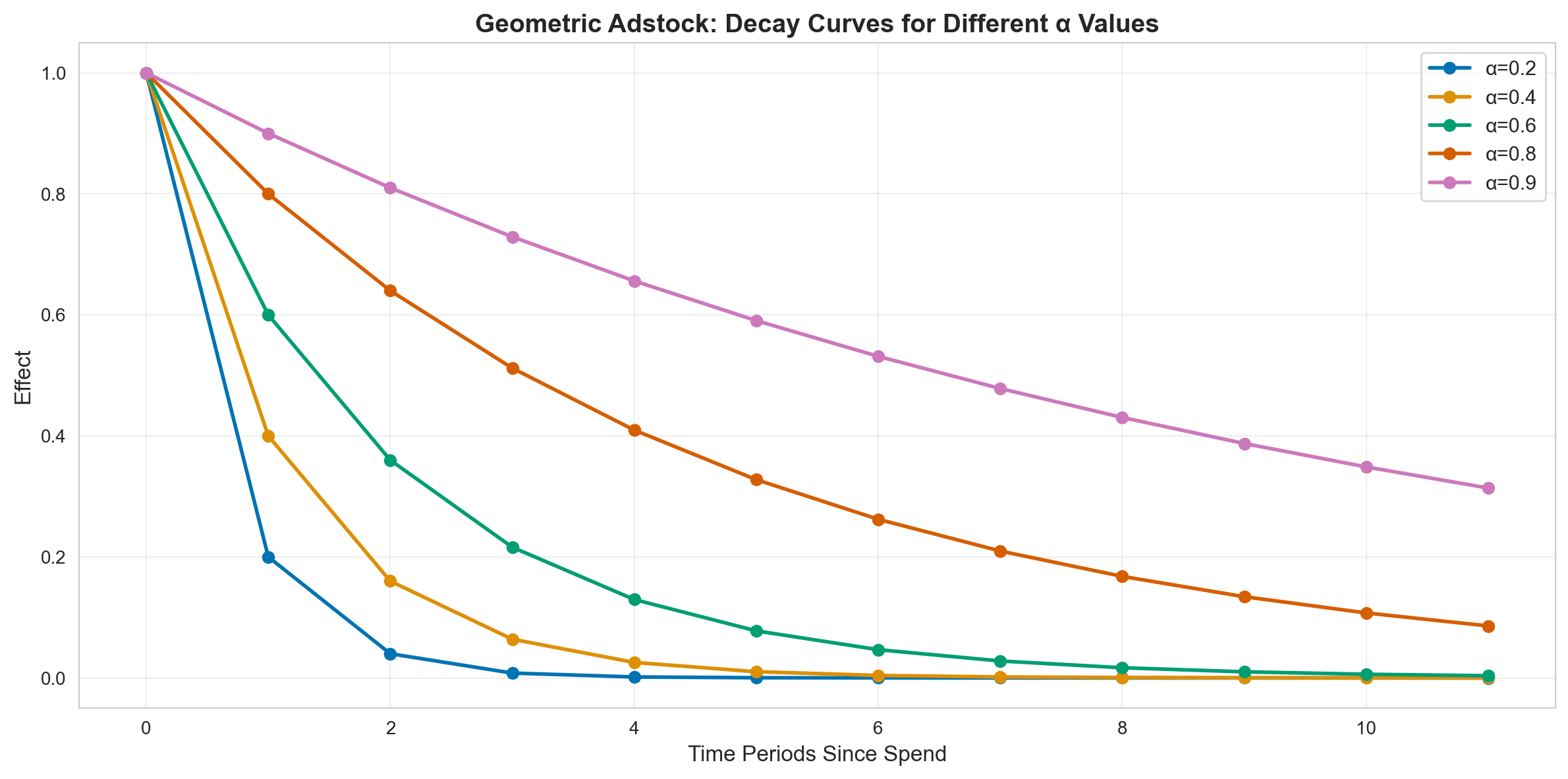
Key Takeaways from Geometric Adstock Decay Curves#
Decay Speed & Duration#
α = 0.2: Effect drops to ~20% after 1 period, nearly zero by week 5
α = 0.4: Effect at ~40% after 1 period, reaches ~1% by week 8
α = 0.6: Effect at ~60% after 1 period, still ~10% at week 5
α = 0.8: Effect at ~80% after 1 period, ~17% remains at week 8
α = 0.9: Effect at ~90% after 1 period, ~35% remains at week 10
Practical Implications#
Low α (0.2-0.4): Performance Marketing
Use for search ads, display ads, direct response campaigns
Spending $1 today has minimal impact beyond 1-2 weeks
Requires consistent, frequent spend to maintain effects
Quick wins but no lasting memory
Medium α (0.5-0.7): Social & Video
Common for social media, video ads, content marketing
Effects last 4-6 weeks with meaningful carryover
Balanced between immediate impact and memory effects
Moderate persistence allows for less aggressive spending
High α (0.8-0.9): Brand & Traditional Media
Brand campaigns, TV, radio, out-of-home advertising
Effects persist for months with strong memory
Can maintain impact with less frequent spending
Long-term investment in brand awareness
Apply Geometric Adstock to Channel Data#
Now that we understand how geometric adstock decay curves work in theory, let’s see what happens when we apply this transformation to real marketing spend data.
What We’re Doing#
We’ll take the raw weekly spend from our two marketing channels (x1 and x2) and transform them using geometric adstock with α = 0.5 (moderate decay). This represents a realistic scenario where advertising effects carry over for several weeks, roughly 50% of the impact remains after one week, 25% after two weeks, and so on.
Why This Matters#
Remember, in the raw data, a spike in spend only appears in that single week. But in reality, that advertising doesn’t just create impact on the day it runs. It creates memories in consumers’ minds that influence their behavior for weeks afterward. The adstock transformation adjusts our spend data to reflect this cumulative, lingering effect.
What to Look For#
When we compare the original spend to the adstocked spend, you’ll notice:
Smoothing: The adstocked curves are smoother than the raw spend because each week’s value incorporates carryover from previous weeks
Elevated Baselines: After periods of high spend, the adstocked values remain elevated even when spend drops to zero—this is the “memory effect”
Delayed Peaks: The peak adstocked values may occur slightly after the peak raw spend, as the full effect accumulates over time
Realistic Impact: The adstocked spend represents what the effective advertising pressure looks like from a consumer’s perspective
This transformation is what we’ll actually feed into our MMM model. Instead of assuming that $100 spent in week 5 only affects sales in week 5, we’re acknowledging that it affects sales in weeks 5, 6, 7… with diminishing impact.
Note
We will follow this process for each type of Adstock transformation throughout the notebook. The process will include exploring the different curve behaviors as well as transforming our media spend with those behaviors.
# Apply geometric adstock with alpha=0.5 (moderate decay)
alpha = 0.5
x1_adstocked_geo = adstock_timeseries(
    data["x1"].values, geometric_adstock, alpha=alpha, l_max=12, normalize=True
)
x2_adstocked_geo = adstock_timeseries(
    data["x2"].values, geometric_adstock, alpha=alpha, l_max=12, normalize=True
)

# Visualize original vs adstocked spend
fig, axes = plt.subplots(2, 1, figsize=(14, 10))

# Channel x1
ax1 = axes[0]
ax1.plot(
    data.index,
    data["x1"],
    label="Original Spend",
    linewidth=2,
    alpha=0.7,
    color=COLOR_CH1,
)
ax1.plot(
    data.index,
    x1_adstocked_geo,
    label=f"Adstocked (α={alpha})",
    linewidth=2,
    linestyle="--",
    color=CB_COLORS[7],
)
ax1.set_title(
    "Channel x1: Original vs Geometric Adstocked Spend", fontsize=14, fontweight="bold"
)
ax1.set_ylabel("Value", fontsize=12)
ax1.legend(fontsize=11)
ax1.grid(True, alpha=0.3)

# Channel x2
ax2 = axes[1]
ax2.plot(
    data.index,
    data["x2"],
    label="Original Spend",
    linewidth=2,
    alpha=0.7,
    color=COLOR_CH2,
)
ax2.plot(
    data.index,
    x2_adstocked_geo,
    label=f"Adstocked (α={alpha})",
    linewidth=2,
    linestyle="--",
    color=CB_COLORS[7],
)
ax2.set_title(
    "Channel x2: Original vs Geometric Adstocked Spend", fontsize=14, fontweight="bold"
)
ax2.set_xlabel("Week Index", fontsize=12)
ax2.set_ylabel("Value", fontsize=12)
ax2.legend(fontsize=11)
ax2.grid(True, alpha=0.3)

plt.tight_layout()
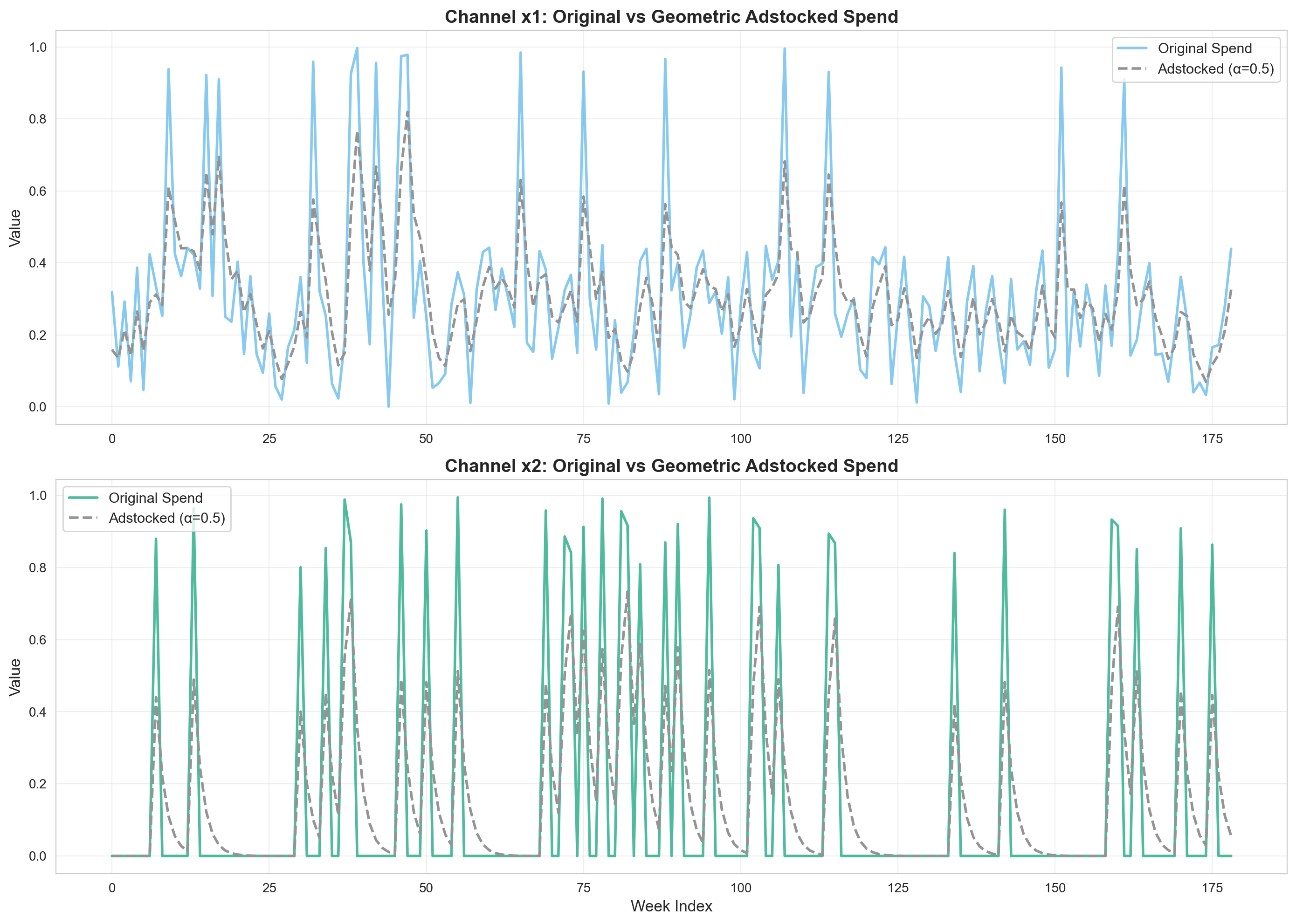
Key Observations:
The adstocked spend is smoother than the original, showing carryover effects
Peaks in spend create lingering effects in subsequent periods
The transformation captures how today’s advertising continues to influence tomorrow’s sales
2. Delayed Adstock#
Overview#
Delayed adstock extends geometric adstock by adding a delay parameter (\(\theta\)) that shifts when the peak effect occurs.
Mathematical Form#
Delayed geometric adstock builds on geometric adstock by adding in a delay \(\theta\) before the maximum adstock is observed (this happens at week 0 for the plain geometric decay).
It also adds a maximum duration for the carryover/adstock \(L_{max}\), such that adstock after this point is 0.
The delayed geometric adstock function takes the following form:
Where:
\(\tilde{x}_t\) is the transformed value at time \(t\) after applying the delayed adstock transformation
\(\alpha\) is the retention rate of the ad effect
\(\theta\) represents the delay before the peak effect occurs
\(L_{max}\) is the maximum duration of the carryover effect
When to Use#
Broadcast media (TV, radio) where impact doesn’t happen immediately
Out-of-home advertising (billboards) with gradual awareness build-up
Awareness campaigns where recognition takes time to develop
When there’s a lag between exposure and action (e.g., B2B marketing)
Brand campaigns rather than performance marketing
Parameters#
alpha: Retention rate (0-1)theta: Delay parameter (higher = more delay)l_max: Maximum lag periods
# Create Delayed Adstock instance
delayed = DelayedAdstock(l_max=12, normalize=True)

print("Delayed Adstock Configuration:")
print(delayed)
Delayed Adstock Configuration:
DelayedAdstock(prefix='adstock', l_max=12, normalize=True, mode='After', priors={'alpha': Prior("Beta", alpha=1, beta=3), 'theta': Prior("HalfNormal", sigma=1)})
Decay Curves for Different Delay (θ) Values#
fig, axes = plt.subplots(1, 2, figsize=(16, 6))

# Test different theta values with fixed alpha
alpha = 0.6
thetas = [0, 1, 2, 3, 4]
l_max = 12

impulse = np.zeros(l_max)
impulse[0] = 1.0

# Left plot: varying theta
for theta in thetas:
    result = delayed_adstock(
        ptx.as_xtensor(impulse, dims=("time",)),
        alpha=alpha,
        theta=theta,
        l_max=l_max,
        normalize=False,
        dim="time",
    )
    axes[0].plot(
        range(l_max), result.eval(), marker="o", linewidth=2, label=f"θ={theta}"
    )

axes[0].set_xlabel("Time Periods Since Spend", fontsize=12)
axes[0].set_ylabel("Effect", fontsize=12)
axes[0].set_title(
    f"Delayed Adstock: Effect of θ (α={alpha})", fontsize=14, fontweight="bold"
)
axes[0].legend(fontsize=11)
axes[0].grid(True, alpha=0.3)

# Right plot: varying alpha with fixed theta
theta = 2
alphas = [0.3, 0.5, 0.7, 0.9]

for alpha in alphas:
    result = delayed_adstock(
        ptx.as_xtensor(impulse, dims=("time",)),
        alpha=alpha,
        theta=theta,
        l_max=l_max,
        normalize=False,
        dim="time",
    )
    axes[1].plot(
        range(l_max), result.eval(), marker="o", linewidth=2, label=f"α={alpha}"
    )

axes[1].set_xlabel("Time Periods Since Spend", fontsize=12)
axes[1].set_ylabel("Effect", fontsize=12)
axes[1].set_title(
    f"Delayed Adstock: Effect of α (θ={theta})", fontsize=14, fontweight="bold"
)
axes[1].legend(fontsize=11)
axes[1].grid(True, alpha=0.3)

plt.tight_layout()
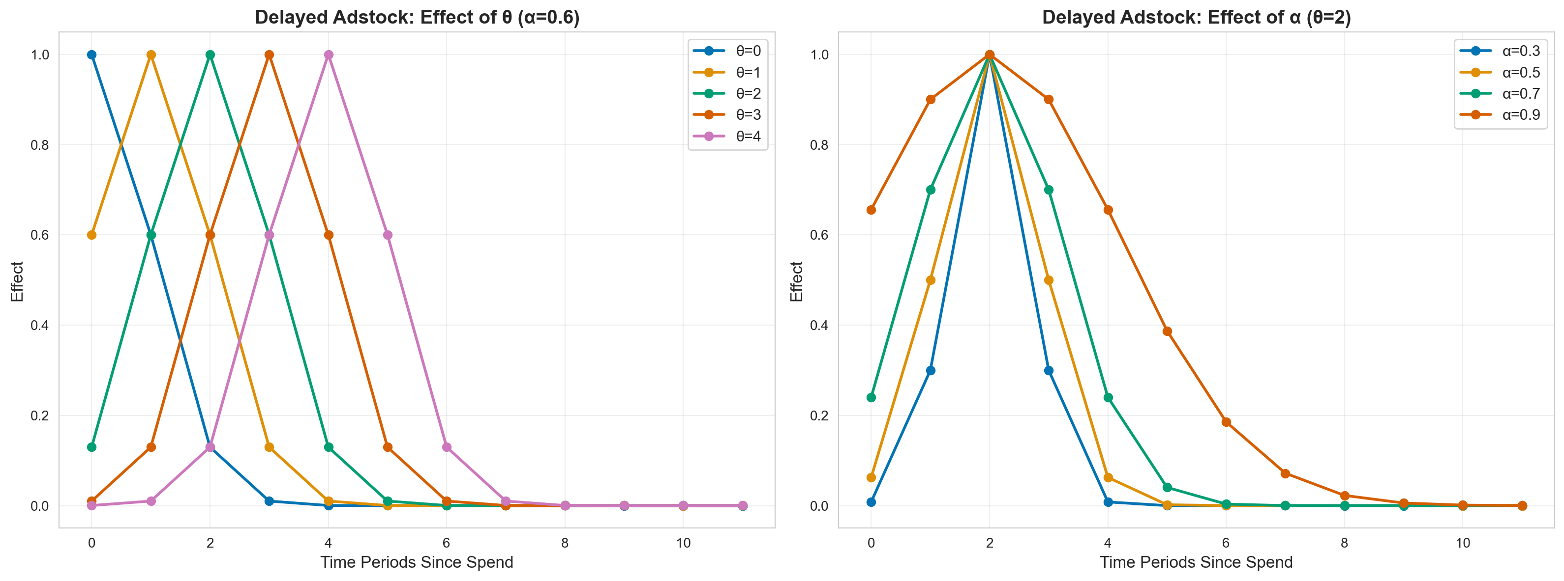
Key Takeaways from Delayed Adstock#
1. Decay Speed & Duration#
Effect of Delay Parameter (θ):
θ = 0: No delay, identical to geometric adstock (immediate peak)
θ = 1: Peak effect occurs 1 period after spend
θ = 2: Peak effect occurs 2 periods after spend
θ = 3-4: Peak effect occurs 3-4 periods after spend, creating significant lag
Effect of Retention (α) with θ=2:
α = 0.3: Fast decay after delayed peak, effects dissipate within 5-6 periods
α = 0.5: Moderate decay, effects last 7-8 periods after peak
α = 0.7: Slow decay, effects persist 9-10 periods with sustained impact
α = 0.9: Very slow decay, effects remain strong even 10+ periods after peak
2. Practical Implications#
Low θ (0-1): Slight Delay Channels
Online video ads where impact builds 1 week after viewing
Social media campaigns with next-day engagement
Email marketing with short consideration periods
Quick response but not instantaneous
Medium θ (2-3): Moderate Delay Channels
TV advertising where brand awareness converts to action after 2-3 weeks
Out-of-home (billboard) advertising with gradual recognition
B2B marketing with typical sales cycles
Awareness campaigns that need time to penetrate
High θ (4+): Long Delay Channels
Brand building campaigns with very long awareness-to-action cycles
Educational content marketing
PR campaigns where sentiment shifts slowly
Complex B2B sales with extended decision-making
Combining θ and α:
High θ + Low α: Sharp peak after delay, then rapid drop-off (promotional events)
High θ + High α: Delayed peak with long-lasting sustained effects (traditional brand advertising)
Low θ + Low α: Quick peak, quick fade (performance marketing with slight delay)
Apply Delayed Adstock to Channel Data#
# Apply delayed adstock with moderate delay and decay
alpha = 0.6
theta = 2
x1_adstocked_delayed = adstock_timeseries(
    data["x1"].values,
    delayed_adstock,
    alpha=alpha,
    theta=theta,
    l_max=12,
    normalize=True,
)
x2_adstocked_delayed = adstock_timeseries(
    data["x2"].values,
    delayed_adstock,
    alpha=alpha,
    theta=theta,
    l_max=12,
    normalize=True,
)

# Visualize
fig, axes = plt.subplots(2, 1, figsize=(14, 10))

# Channel x1
ax1 = axes[0]
ax1.plot(
    data.index,
    data["x1"],
    label="Original Spend",
    linewidth=2,
    alpha=0.7,
    color=COLOR_CH1,
)
ax1.plot(
    data.index,
    x1_adstocked_delayed,
    label=f"Delayed Adstock (α={alpha}, θ={theta})",
    linewidth=2,
    linestyle="--",
    color=CB_COLORS[7],
)
ax1.set_title(
    "Channel x1: Original vs Delayed Adstocked Spend", fontsize=14, fontweight="bold"
)
ax1.set_ylabel("Value", fontsize=12)
ax1.legend(fontsize=11)
ax1.grid(True, alpha=0.3)

# Channel x2
ax2 = axes[1]
ax2.plot(
    data.index,
    data["x2"],
    label="Original Spend",
    linewidth=2,
    alpha=0.7,
    color=COLOR_CH2,
)
ax2.plot(
    data.index,
    x2_adstocked_delayed,
    label=f"Delayed Adstock (α={alpha}, θ={theta})",
    linewidth=2,
    linestyle="--",
    color=CB_COLORS[7],
)
ax2.set_title(
    "Channel x2: Original vs Delayed Adstocked Spend", fontsize=14, fontweight="bold"
)
ax2.set_xlabel("Week Index", fontsize=12)
ax2.set_ylabel("Value", fontsize=12)
ax2.legend(fontsize=11)
ax2.grid(True, alpha=0.3)

plt.tight_layout()
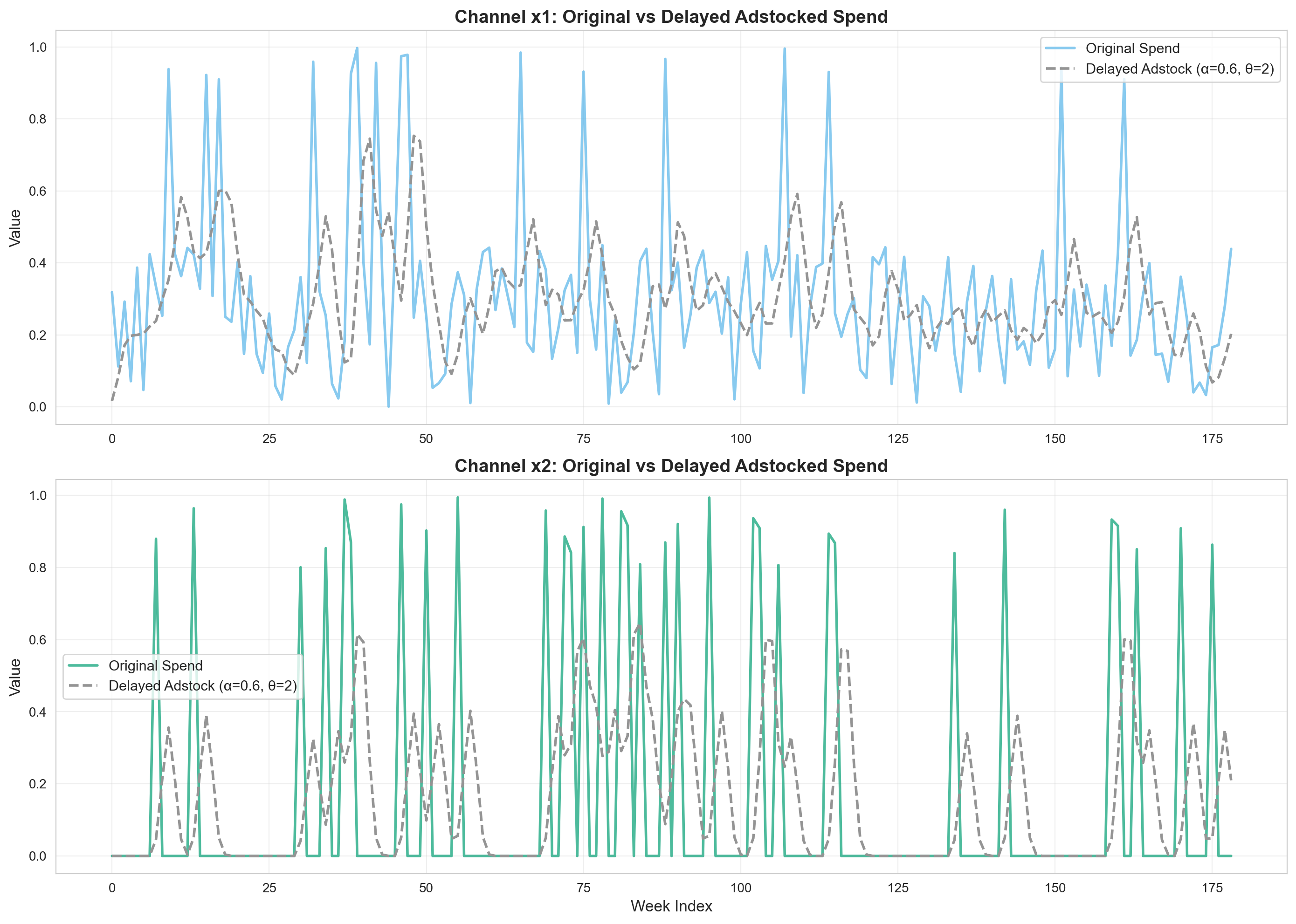
Key Observations:
The delay creates a lag between spend and its full effect
Notice how effects are shifted forward in time compared to geometric adstock
Useful when you expect marketing to take time to “sink in”
3. Weibull CDF Adstock#
Overview#
Weibull CDF adstock uses the cumulative distribution function, creating an S-shaped curve where effects build up gradually.
Mathematical Form#
The Weibull CDF is a function depending on two variables, \(k\) (known as the shape) and \(\lambda\) (known as the scale).
The idea is closely related to geometric adstock but with one important difference : the rate of decay (what we called \(\alpha\) in the geometric adstock equation) is no longer fixed. Instead it’s time-dependent.
The Weibull CDF adstock function therefore takes the form :
where \(\alpha_t\) is now a function of time \(t\)
The Weibull CDF is actually used to build the \(\alpha_t\)’s, and it takes the form :
Then, \(\alpha_t\) is computed as :
When to Use#
Brand building campaigns with cumulative awareness
Long-term PR campaigns where impact accumulates
Content marketing that builds authority over time
Educational campaigns with gradual learning
When effects are cumulative and slow-building
Word-of-mouth marketing that spreads gradually
Parameters#
lam: Scale parameter (λ)k: Shape parameterl_max: Maximum lag periods
# Create Weibull CDF Adstock instance
weibull_cdf = WeibullCDFAdstock(l_max=12, normalize=True)

print("Weibull CDF Adstock Configuration:")
print(weibull_cdf)
Weibull CDF Adstock Configuration:
WeibullCDFAdstock(prefix='adstock', l_max=12, normalize=True, mode='After', priors={'lam': Prior("Gamma", mu=2, sigma=2.5), 'k': Prior("Gamma", mu=2, sigma=2.5)})
Decay Curves for Different λ and k Values#
fig, axes = plt.subplots(1, 2, figsize=(16, 6))

l_max = 12
impulse = np.zeros(l_max)
impulse[0] = 1.0

# Left plot: varying lambda (scale)
k = 2
lambdas = [0.5, 1, 2, 3, 4]

for lam in lambdas:
    result = weibull_adstock(
        ptx.as_xtensor(impulse, dims=("time",)),
        lam=lam,
        k=k,
        l_max=l_max,
        type=WeibullType.CDF,
        normalize=False,
        dim="time",
    )
    axes[0].plot(range(l_max), result.eval(), marker="o", linewidth=2, label=f"λ={lam}")

axes[0].set_xlabel("Time Periods Since Spend", fontsize=12)
axes[0].set_ylabel("Cumulative Effect", fontsize=12)
axes[0].set_title(
    f"Weibull CDF Adstock: Effect of λ (k={k})", fontsize=14, fontweight="bold"
)
axes[0].legend(fontsize=11)
axes[0].grid(True, alpha=0.3)

# Right plot: varying k (shape)
lam = 2
ks = [0.5, 1, 2, 3, 4]

for k in ks:
    result = weibull_adstock(
        ptx.as_xtensor(impulse, dims=("time",)),
        lam=lam,
        k=k,
        l_max=l_max,
        type=WeibullType.CDF,
        normalize=False,
        dim="time",
    )
    axes[1].plot(range(l_max), result.eval(), marker="o", linewidth=2, label=f"k={k}")

axes[1].set_xlabel("Time Periods Since Spend", fontsize=12)
axes[1].set_ylabel("Cumulative Effect", fontsize=12)
axes[1].set_title(
    f"Weibull CDF Adstock: Effect of k (λ={lam})", fontsize=14, fontweight="bold"
)
axes[1].legend(fontsize=11)
axes[1].grid(True, alpha=0.3)

plt.tight_layout()
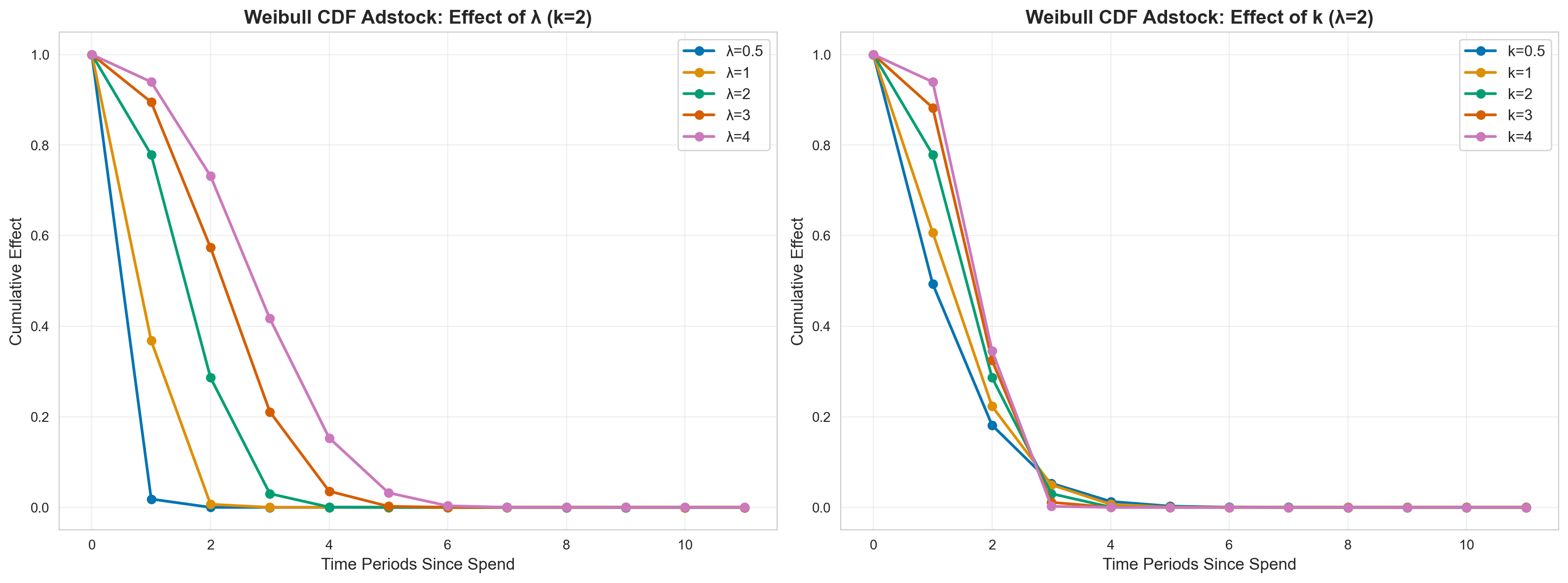
Key Takeaways from Weibull CDF Adstock#
1. Decay Speed & Duration#
Effect of Scale Parameter (λ) with k=2:
λ = 0.5: Rapid S-curve buildup, reaches 90%+ effect by period 1-2
λ = 1: Moderate buildup, reaches plateau around period 3-4
λ = 2: Gradual buildup, reaches plateau around period 5-6
λ = 3-4: Very slow buildup, takes 10+ periods to reach plateau
Effect of Shape Parameter (k) with λ=2:
k = 0.5: Extremely gradual S-curve, very slow initial buildup
k = 1: Linear-like buildup (exponential distribution)
k = 2: Classic S-shaped curve with inflection point
k = 3-4: Steeper S-curve, faster transition from buildup to plateau
Cumulative Nature:
Effects accumulate over time rather than decay
Creates a saturating effect where impact plateaus
Later periods maintain near-100% of cumulative effect
2. Practical Implications#
Low λ (0.5-1): Fast Buildup Channels
Word-of-mouth campaigns that quickly reach saturation
Viral content with rapid but capped spread
Network effects that accelerate quickly
Local market awareness that saturates fast
Medium λ (2-3): Gradual Buildup Channels
Content marketing building authority over months
SEO efforts with cumulative ranking improvements
Brand awareness campaigns in new markets
PR campaigns gradually building reputation
Podcast advertising with growing listener base
High λ (4+): Very Slow Buildup Channels
Long-term brand equity building
Educational initiatives with slow adoption
Category creation marketing
Institutional reputation building
Shape Parameter (k) Implications:
Low k: Use when awareness builds very gradually at first
High k: Use when there’s a tipping point where awareness accelerates then plateaus
k ≈ 2: Good default for most cumulative brand-building scenarios
Apply Weibull CDF Adstock to Channel Data#
# Apply Weibull CDF adstock
lam = 2
k = 2
x1_adstocked_wcdf = adstock_timeseries(
    data["x1"].values,
    weibull_adstock,
    lam=lam,
    k=k,
    l_max=12,
    type=WeibullType.CDF,
    normalize=True,
)
x2_adstocked_wcdf = adstock_timeseries(
    data["x2"].values,
    weibull_adstock,
    lam=lam,
    k=k,
    l_max=12,
    type=WeibullType.CDF,
    normalize=True,
)

# Visualize
fig, axes = plt.subplots(2, 1, figsize=(14, 10))

# Channel x1
ax1 = axes[0]
ax1.plot(
    data.index,
    data["x1"],
    label="Original Spend",
    linewidth=2,
    alpha=0.7,
    color=COLOR_CH1,
)
ax1.plot(
    data.index,
    x1_adstocked_wcdf,
    label=f"Weibull CDF (λ={lam}, k={k})",
    linewidth=2,
    linestyle="--",
    color=CB_COLORS[7],
)
ax1.set_title(
    "Channel x1: Original vs Weibull CDF Adstocked Spend",
    fontsize=14,
    fontweight="bold",
)
ax1.set_ylabel("Value", fontsize=12)
ax1.legend(fontsize=11)
ax1.grid(True, alpha=0.3)

# Channel x2
ax2 = axes[1]
ax2.plot(
    data.index,
    data["x2"],
    label="Original Spend",
    linewidth=2,
    alpha=0.7,
    color=COLOR_CH2,
)
ax2.plot(
    data.index,
    x2_adstocked_wcdf,
    label=f"Weibull CDF (λ={lam}, k={k})",
    linewidth=2,
    linestyle="--",
    color=CB_COLORS[7],
)
ax2.set_title(
    "Channel x2: Original vs Weibull CDF Adstocked Spend",
    fontsize=14,
    fontweight="bold",
)
ax2.set_xlabel("Week Index", fontsize=12)
ax2.set_ylabel("Value", fontsize=12)
ax2.legend(fontsize=11)
ax2.grid(True, alpha=0.3)

plt.tight_layout()
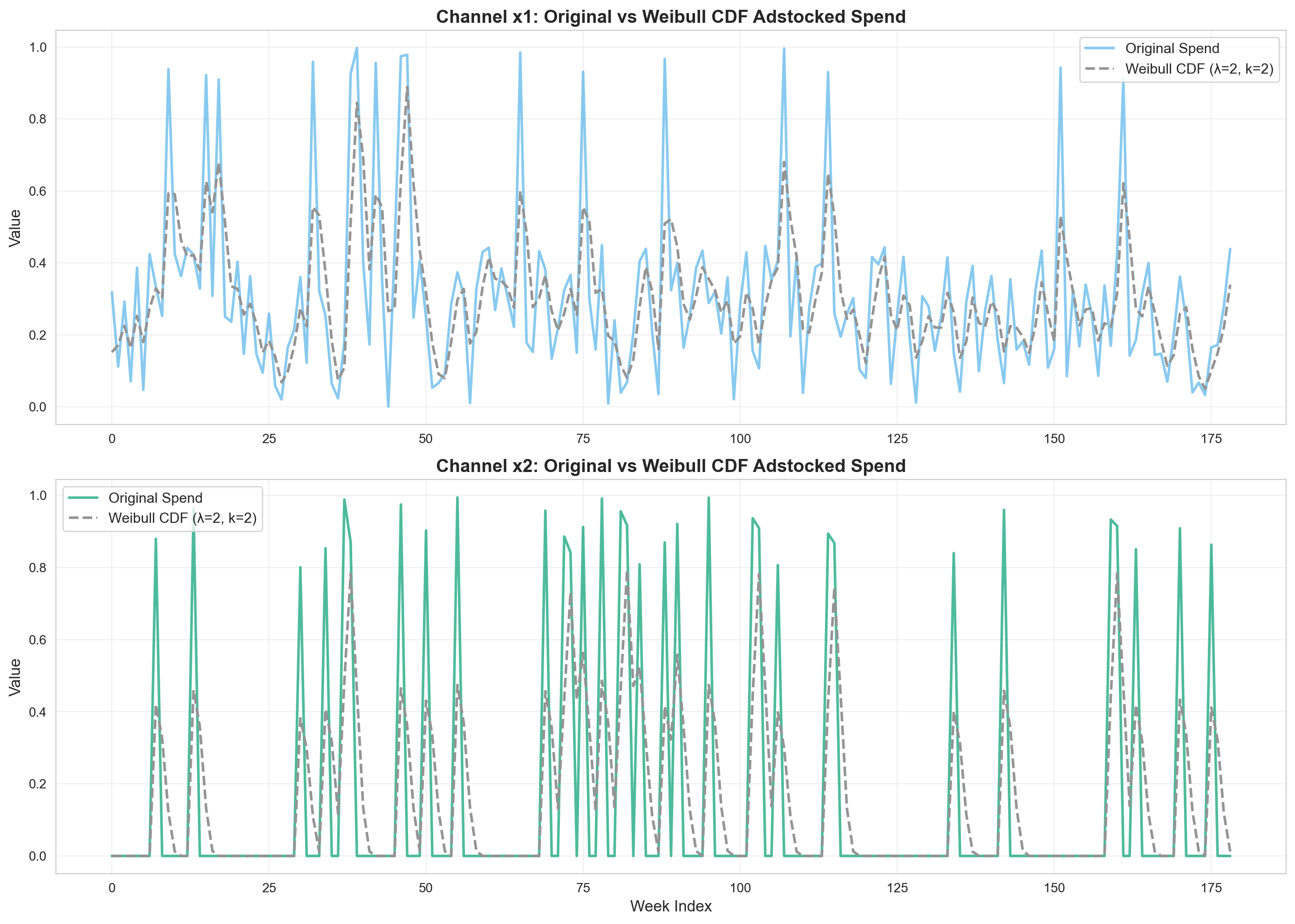
Key Observations:
Weibull CDF shows gradual buildup of marketing effects
Effects accumulate rather than immediately peak
Particularly useful for long-term brand building
4. Weibull PDF Adstock#
Overview#
Weibull PDF adstock uses the probability density function of the Weibull distribution, creating a peak effect followed by decay.
Mathematical Form#
The Weibull PDF is a function depending on two variables, \(k\) (shape) and \(\lambda\) (scale) and the same remarks for Weibull CDF apply to Weibull PDF.
The key difference is that Weibull PDF allows for lagged effects to be taken into account - the time delay effect.
The Weibull PDF adstock function therefore takes the form :
where \(\alpha_t\) is now a function of time \(t\)
The Weibull PDF is actually used to build the \(\alpha_t\)’s, and it takes the form :
When to Use#
Product launches where interest peaks then declines
Promotional campaigns with initial excitement that fades
Event-driven marketing (sales, holidays)
Influencer marketing where buzz builds then dissipates
When you expect maximum impact is not immediate but occurs after some delay
Viral content that peaks before declining
Parameters#
lam: Scale parameter (λ) - controls peak timingk: Shape parameter - controls curve shapel_max: Maximum lag periods
# Create Weibull PDF Adstock instance
weibull_pdf = WeibullPDFAdstock(l_max=12, normalize=True)

print("Weibull PDF Adstock Configuration:")
print(weibull_pdf)
Weibull PDF Adstock Configuration:
WeibullPDFAdstock(prefix='adstock', l_max=12, normalize=True, mode='After', priors={'lam': Prior("Gamma", mu=2, sigma=1), 'k': Prior("Gamma", mu=3, sigma=1)})
Decay Curves for Different λ and k Values#
from pymc_marketing.mmm.transformers import WeibullType, weibull_adstock

fig, axes = plt.subplots(1, 2, figsize=(16, 6))

l_max = 12
impulse = np.zeros(l_max)
impulse[0] = 1.0

# Left plot: varying lambda (scale)
k = 2
lambdas = [0.5, 1, 2, 3, 4]

for lam in lambdas:
    result = weibull_adstock(
        ptx.as_xtensor(impulse, dims=("time",)),
        lam=lam,
        k=k,
        l_max=l_max,
        type=WeibullType.PDF,
        normalize=False,
        dim="time",
    )
    axes[0].plot(range(l_max), result.eval(), marker="o", linewidth=2, label=f"λ={lam}")

axes[0].set_xlabel("Time Periods Since Spend", fontsize=12)
axes[0].set_ylabel("Effect", fontsize=12)
axes[0].set_title(
    f"Weibull PDF Adstock: Effect of λ (k={k})", fontsize=14, fontweight="bold"
)
axes[0].legend(fontsize=11)
axes[0].grid(True, alpha=0.3)

# Right plot: varying k (shape)
lam = 2
ks = [0.5, 1, 2, 3, 4]

for k in ks:
    result = weibull_adstock(
        ptx.as_xtensor(impulse, dims=("time",)),
        lam=lam,
        k=k,
        l_max=l_max,
        type=WeibullType.PDF,
        normalize=False,
        dim="time",
    )
    axes[1].plot(range(l_max), result.eval(), marker="o", linewidth=2, label=f"k={k}")

axes[1].set_xlabel("Time Periods Since Spend", fontsize=12)
axes[1].set_ylabel("Effect", fontsize=12)
axes[1].set_title(
    f"Weibull PDF Adstock: Effect of k (λ={lam})", fontsize=14, fontweight="bold"
)
axes[1].legend(fontsize=11)
axes[1].grid(True, alpha=0.3)

plt.tight_layout()
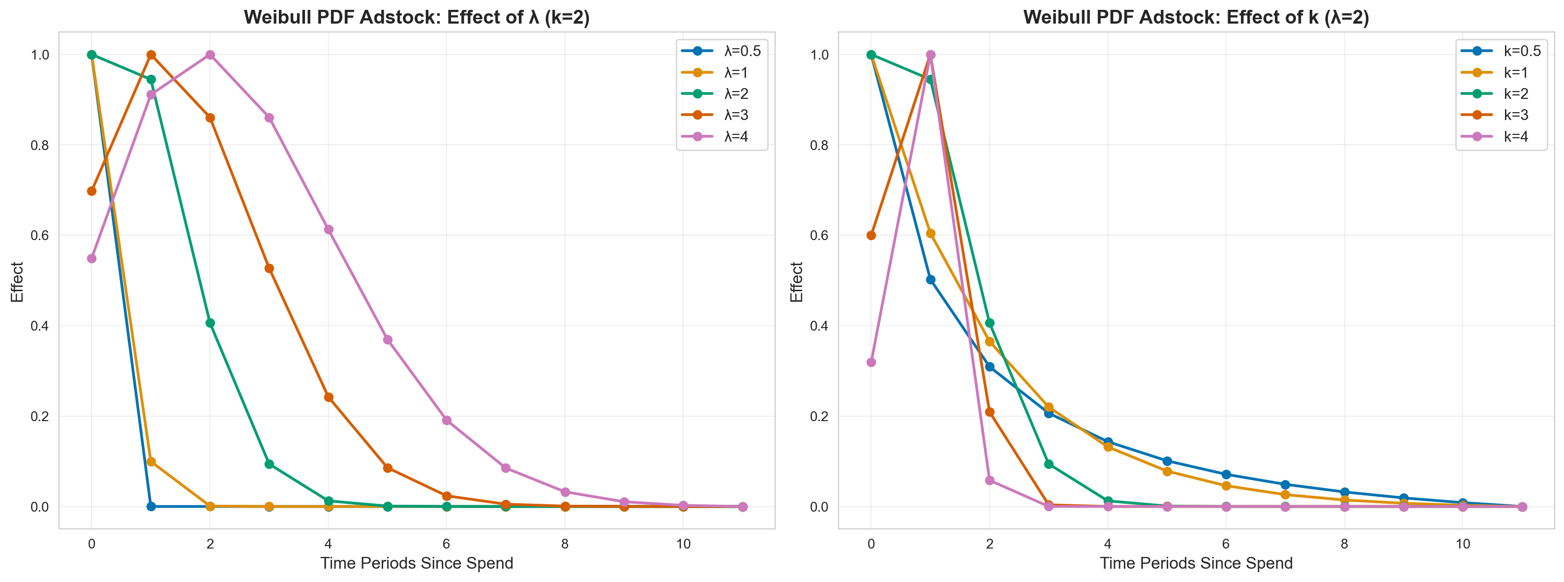
Key Takeaways from Weibull CDF Adstock#
1. Decay Speed & Duration#
Effect of Scale Parameter (λ) with k=2:
λ = 0.5: Rapid S-curve buildup, reaches 90%+ effect by period 2-3
λ = 1: Moderate buildup, reaches plateau around period 4-5
λ = 2: Gradual buildup, reaches plateau around period 7-8
λ = 3-4: Very slow buildup, takes 10+ periods to reach plateau
Effect of Shape Parameter (k) with λ=2:
k = 0.5: Extremely gradual S-curve, very slow initial buildup
k = 1: Linear-like buildup (exponential distribution)
k = 2: Classic S-shaped curve with inflection point
k = 3-4: Steeper S-curve, faster transition from buildup to plateau
Cumulative Nature:
Effects accumulate over time rather than decay
Creates a saturating effect where impact plateaus
Later periods maintain near-100% of cumulative effect
2. Practical Implications#
Low λ (0.5-1): Fast Buildup Channels
Word-of-mouth campaigns that quickly reach saturation
Viral content with rapid but capped spread
Network effects that accelerate quickly
Local market awareness that saturates fast
Medium λ (2-3): Gradual Buildup Channels
Content marketing building authority over months
SEO efforts with cumulative ranking improvements
Brand awareness campaigns in new markets
PR campaigns gradually building reputation
Podcast advertising with growing listener base
High λ (4+): Very Slow Buildup Channels
Long-term brand equity building
Educational initiatives with slow adoption
Category creation marketing
Institutional reputation building
Shape Parameter (k) Implications:
Low k: Use when awareness builds very gradually at first
High k: Use when there’s a tipping point where awareness accelerates then plateaus
k ≈ 2: Good default for most cumulative brand-building scenarios
Apply Weibull PDF Adstock to Channel Data#
# Apply Weibull PDF adstock
lam = 2
k = 2
x1_adstocked_wpdf = adstock_timeseries(
    data["x1"].values,
    weibull_adstock,
    lam=lam,
    k=k,
    l_max=12,
    type=WeibullType.PDF,
    normalize=True,
)
x2_adstocked_wpdf = adstock_timeseries(
    data["x2"].values,
    weibull_adstock,
    lam=lam,
    k=k,
    l_max=12,
    type=WeibullType.PDF,
    normalize=True,
)

# Visualize
fig, axes = plt.subplots(2, 1, figsize=(14, 10))

# Channel x1
ax1 = axes[0]
ax1.plot(
    data.index,
    data["x1"],
    label="Original Spend",
    linewidth=2,
    alpha=0.7,
    color=COLOR_CH1,
)
ax1.plot(
    data.index,
    x1_adstocked_wpdf,
    label=f"Weibull PDF (λ={lam}, k={k})",
    linewidth=2,
    linestyle="--",
    color=CB_COLORS[7],
)
ax1.set_title(
    "Channel x1: Original vs Weibull PDF Adstocked Spend",
    fontsize=14,
    fontweight="bold",
)
ax1.set_ylabel("Value", fontsize=12)
ax1.legend(fontsize=11)
ax1.grid(True, alpha=0.3)

# Channel x2
ax2 = axes[1]
ax2.plot(
    data.index,
    data["x2"],
    label="Original Spend",
    linewidth=2,
    alpha=0.7,
    color=COLOR_CH2,
)
ax2.plot(
    data.index,
    x2_adstocked_wpdf,
    label=f"Weibull PDF (λ={lam}, k={k})",
    linewidth=2,
    linestyle="--",
    color=CB_COLORS[7],
)
ax2.set_title(
    "Channel x2: Original vs Weibull PDF Adstocked Spend",
    fontsize=14,
    fontweight="bold",
)
ax2.set_xlabel("Week Index", fontsize=12)
ax2.set_ylabel("Value", fontsize=12)
ax2.legend(fontsize=11)
ax2.grid(True, alpha=0.3)

plt.tight_layout()
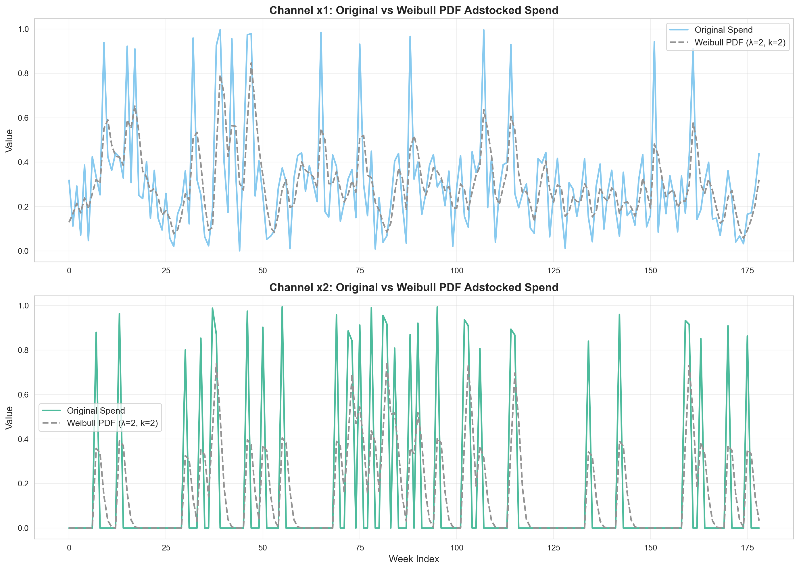
Key Observations:
The Weibull PDF creates a peak effect after the spend
Useful for modeling campaigns where impact builds before declining
Different from geometric where effect is immediate
5. Binomial Adstock#
Overview#
Binomial adstock provides a flexible decay curve based on the binomial distribution.
Mathematical Form#
Binomial adstock assumes that the effect of one unit of spend at time \(t\) is given by:
Where:
\(t\) is the time since the advertising spend (\(0 \le t \le L + 1\))
\(L\) is
l_max, the maximum duration of carryover effect\(\alpha \in (0, 1)\) is the shape parameter controlling the decay curve
Notice that \(f(L + 1) = 0\)
The binomial adstock transformation provides more flexible decay shapes compared to geometric adstock. The \(\alpha\) parameter controls both the shape and the decay rate, allowing for convex and concave decay patterns.
When to Use#
When you need more flexible decay shapes than geometric
Social media advertising with variable decay patterns
Email marketing where engagement varies over time
When geometric adstock is too restrictive
When you want decay to be data-driven rather than assumed
Parameters#
alpha: Shape parameter controlling decay curvel_max: Maximum lag periods
# Create Binomial Adstock instance
binomial = BinomialAdstock(l_max=12, normalize=True)

print("Binomial Adstock Configuration:")
print(binomial)
Binomial Adstock Configuration:
BinomialAdstock(prefix='adstock', l_max=12, normalize=True, mode='After', priors={'alpha': Prior("Beta", alpha=1, beta=3)})
Decay Curves for Different Alpha Values#
fig, ax = plt.subplots(figsize=(12, 6))

alphas = [0.1, 0.3, 0.5, 0.7, 0.9]
l_max = 12

impulse = np.zeros(l_max)
impulse[0] = 1.0

for alpha in alphas:
    result = binomial_adstock(
        ptx.as_xtensor(impulse, dims=("time",)),
        alpha=alpha,
        l_max=l_max,
        normalize=False,
        dim="time",
    )
    ax.plot(range(l_max), result.eval(), marker="o", linewidth=2, label=f"α={alpha}")

ax.set_xlabel("Time Periods Since Spend", fontsize=12)
ax.set_ylabel("Effect", fontsize=12)
ax.set_title(
    "Binomial Adstock: Decay Curves for Different α Values",
    fontsize=14,
    fontweight="bold",
)
ax.legend(fontsize=11)
ax.grid(True, alpha=0.3)
plt.tight_layout()
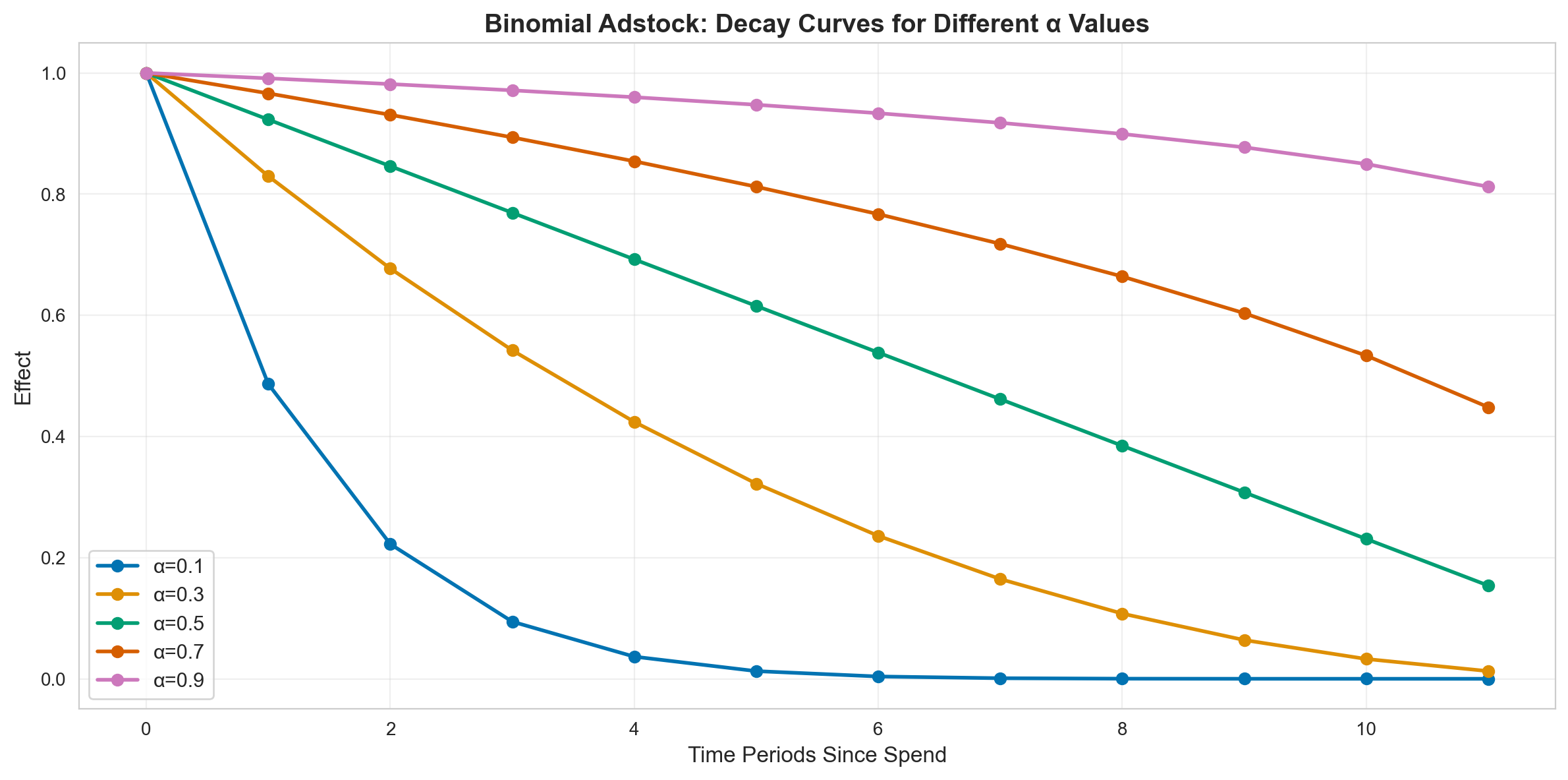
Key Takeaways from Binomial Adstock#
1. Decay Speed & Duration#
Effect of Alpha Parameter:
α = 0.1: Extremely steep, convex decay – effect drops to near-zero by period 2-3
α = 0.3: Steep convex decay, most effect gone by period 4-5
α = 0.5: Moderate convex decay, effects last ~6-7 periods
α = 0.7: Gentle, more linear decay, effects last ~8-9 periods
α = 0.9: Very gentle, nearly linear decay, effects persist 10+ periods
Decay Shape Characteristics:
Low α (0.1-0.3): Strong convex curvature (rapid initial decay, then slower)
Medium α (0.4-0.6): Moderate curvature, balanced decay
High α (0.7-0.9): Near-linear or slightly concave decay
Unique Feature:
Unlike geometric adstock, binomial allows convex decay patterns
Effect decreases faster initially, then tapers off more gently
Provides middle ground between geometric and Weibull patterns
2. Practical Implications#
Low α (0.1-0.3): Rapid Initial Impact Channels
Push notifications with immediate but short-lived response
Flash sales where urgency drives immediate action
Time-sensitive alerts or announcements
Mobile app install campaigns with quick drop-off
Social media ads with high initial engagement, fast fatigue
Medium α (0.4-0.6): Balanced Decay Channels
Standard social media advertising
Display advertising with moderate frequency
Email campaigns with follow-up sequences
Retargeting campaigns
Video ads with moderate recall
High α (0.7-0.9): Sustained Effect Channels
Content marketing with evergreen value
SEO-driven traffic with sustained visibility
Community building initiatives
Brand partnerships with long-term presence
Educational content with lasting utility
When to Use Binomial vs. Geometric:
Use Binomial when you expect initial effect to be stronger than geometric suggests
Use Binomial for channels with quick initial response but lingering secondary effects
Use Binomial when geometric adstock is too rigid and Weibull too complex
Use Binomial as a flexible alternative for model comparison/selection
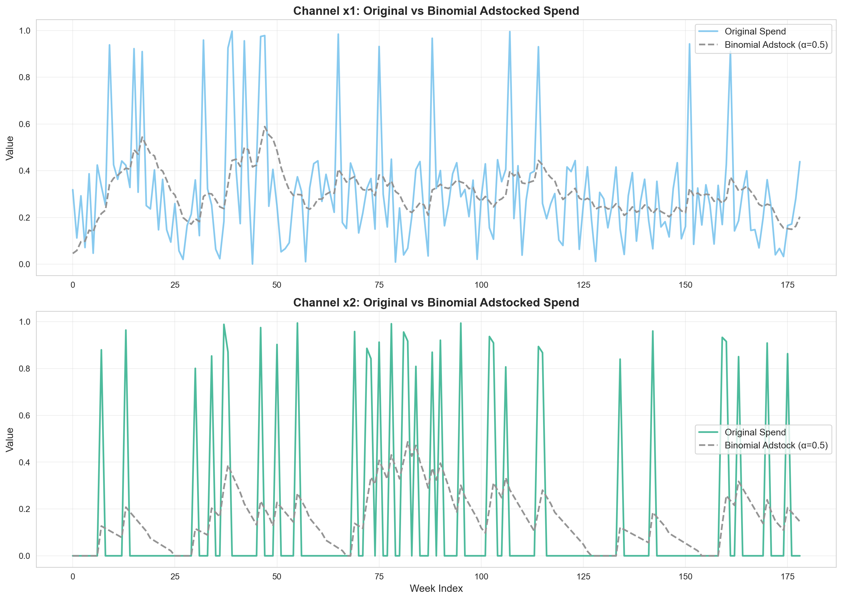
Apply Binomial Adstock to Channel Data#
# Apply binomial adstock
alpha = 0.5
x1_adstocked_binom = adstock_timeseries(
    data["x1"].values, binomial_adstock, alpha=alpha, l_max=12, normalize=True
)
x2_adstocked_binom = adstock_timeseries(
    data["x2"].values, binomial_adstock, alpha=alpha, l_max=12, normalize=True
)

# Visualize
fig, axes = plt.subplots(2, 1, figsize=(14, 10))

# Channel x1
ax1 = axes[0]
ax1.plot(
    data.index,
    data["x1"],
    label="Original Spend",
    linewidth=2,
    alpha=0.7,
    color=COLOR_CH1,
)
ax1.plot(
    data.index,
    x1_adstocked_binom,
    label=f"Binomial Adstock (α={alpha})",
    linewidth=2,
    linestyle="--",
    color=CB_COLORS[7],
)
ax1.set_title(
    "Channel x1: Original vs Binomial Adstocked Spend", fontsize=14, fontweight="bold"
)
ax1.set_ylabel("Value", fontsize=12)
ax1.legend(fontsize=11)
ax1.grid(True, alpha=0.3)

# Channel x2
ax2 = axes[1]
ax2.plot(
    data.index,
    data["x2"],
    label="Original Spend",
    linewidth=2,
    alpha=0.7,
    color=COLOR_CH2,
)
ax2.plot(
    data.index,
    x2_adstocked_binom,
    label=f"Binomial Adstock (α={alpha})",
    linewidth=2,
    linestyle="--",
    color=CB_COLORS[7],
)
ax2.set_title(
    "Channel x2: Original vs Binomial Adstocked Spend", fontsize=14, fontweight="bold"
)
ax2.set_xlabel("Week Index", fontsize=12)
ax2.set_ylabel("Value", fontsize=12)
ax2.legend(fontsize=11)
ax2.grid(True, alpha=0.3)

plt.tight_layout()
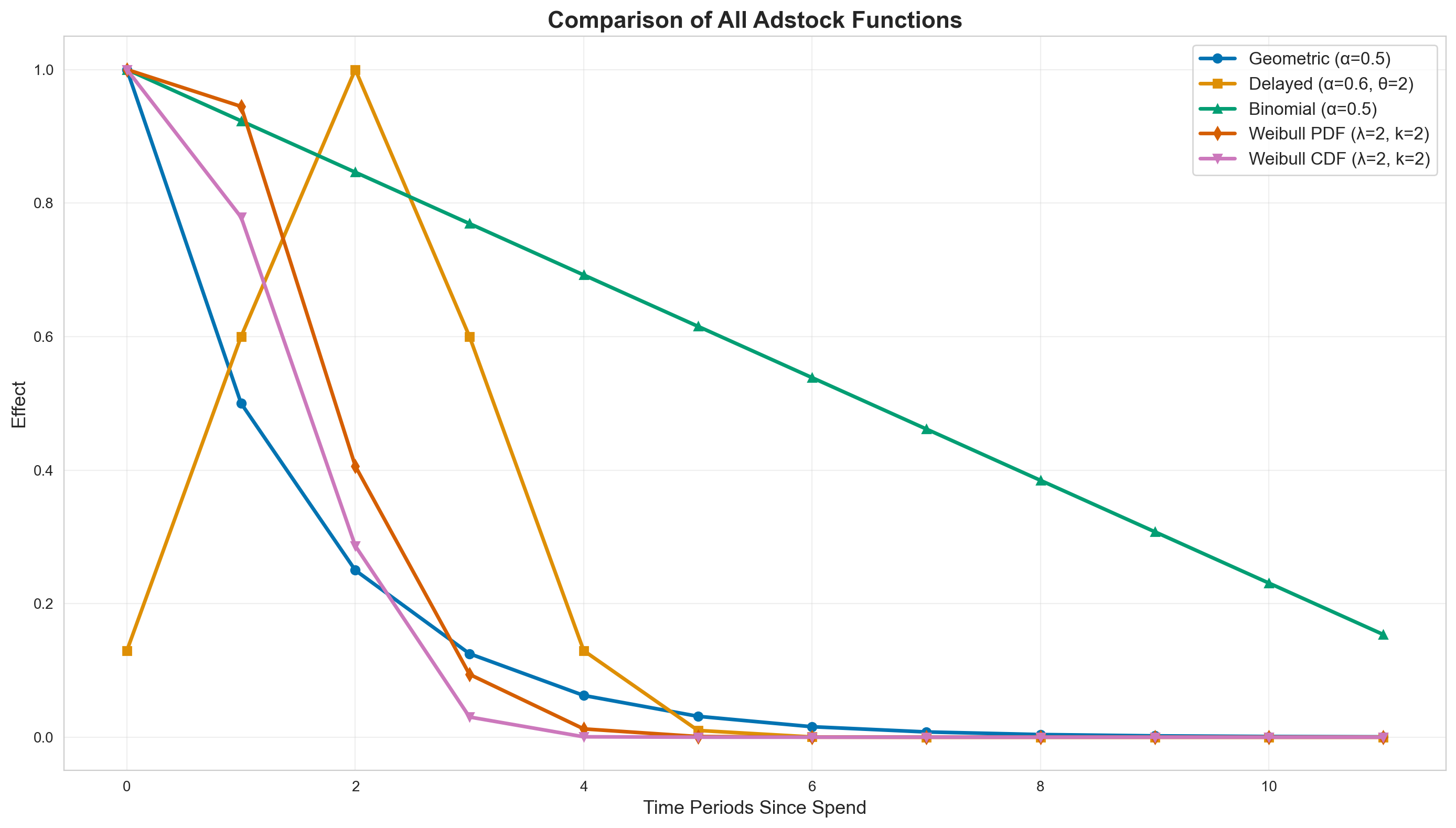
6. Comparison Across All Adstock Functions#
Let’s compare all adstock functions side-by-side to understand their differences:
Decay Curve Comparison#
fig, ax = plt.subplots(figsize=(14, 8))

l_max = 12
impulse = np.zeros(l_max)
impulse[0] = 1.0

# Geometric
geo = geometric_adstock(
    ptx.as_xtensor(impulse, dims=("time",)),
    alpha=0.5,
    l_max=l_max,
    normalize=False,
    dim="time",
).eval()
ax.plot(
    range(l_max),
    geo,
    marker="o",
    linewidth=2.5,
    label="Geometric (α=0.5)",
    markersize=6,
    color=CB_COLORS[0],
)

# Delayed
delayed_result = delayed_adstock(
    ptx.as_xtensor(impulse, dims=("time",)),
    alpha=0.6,
    theta=2,
    l_max=l_max,
    normalize=False,
    dim="time",
).eval()
ax.plot(
    range(l_max),
    delayed_result,
    marker="s",
    linewidth=2.5,
    label="Delayed (α=0.6, θ=2)",
    markersize=6,
    color=CB_COLORS[1],
)

# Binomial
binom = binomial_adstock(
    ptx.as_xtensor(impulse, dims=("time",)),
    alpha=0.5,
    l_max=l_max,
    normalize=False,
    dim="time",
).eval()
ax.plot(
    range(l_max),
    binom,
    marker="^",
    linewidth=2.5,
    label="Binomial (α=0.5)",
    markersize=6,
    color=CB_COLORS[2],
)

# Weibull PDF
wpdf = weibull_adstock(
    ptx.as_xtensor(impulse, dims=("time",)),
    lam=2,
    k=2,
    l_max=l_max,
    type=WeibullType.PDF,
    normalize=False,
    dim="time",
).eval()
ax.plot(
    range(l_max),
    wpdf,
    marker="d",
    linewidth=2.5,
    label="Weibull PDF (λ=2, k=2)",
    markersize=6,
    color=CB_COLORS[3],
)

# Weibull CDF
wcdf = weibull_adstock(
    ptx.as_xtensor(impulse, dims=("time",)),
    lam=2,
    k=2,
    l_max=l_max,
    type=WeibullType.CDF,
    normalize=False,
    dim="time",
).eval()
ax.plot(
    range(l_max),
    wcdf,
    marker="v",
    linewidth=2.5,
    label="Weibull CDF (λ=2, k=2)",
    markersize=6,
    color=CB_COLORS[4],
)

ax.set_xlabel("Time Periods Since Spend", fontsize=13)
ax.set_ylabel("Effect", fontsize=13)
ax.set_title("Comparison of All Adstock Functions", fontsize=16, fontweight="bold")
ax.legend(fontsize=12, loc="best")
ax.grid(True, alpha=0.3)
plt.tight_layout()

print("\nKey Differences:")
print("- Geometric (blue): Immediate peak, exponential decay")
print("- Delayed (orange): Peak shifted forward in time")
print("- Weibull CDF (purple): Gradual S-shaped buildup")
print("- Weibull PDF (red): Peak after delay, then decay")
print("- Binomial (green): Flexible decay shape")
Key Differences:
- Geometric (blue): Immediate peak, exponential decay
- Delayed (orange): Peak shifted forward in time
- Weibull CDF (purple): Gradual S-shaped buildup
- Weibull PDF (red): Peak after delay, then decay
- Binomial (green): Flexible decay shape
Transformed Time Series Comparison#
Now let’s compare how each adstock transformation affects the actual channel spend data over time. This shows the real-world impact of choosing different adstock functions on your marketing data.
# Create subplots with shared x-axis
fig = make_subplots(
    rows=2,
    cols=1,
    subplot_titles=(
        "Channel x1: Comparison of All Adstock Transformations",
        "Channel x2: Comparison of All Adstock Transformations",
    ),
    vertical_spacing=0.12,
    shared_xaxes=True,
)

# Define colors to match the decay curve comparison
colors = {
    "Original": "rgba(0, 0, 0, 0.5)",
    "Geometric": "#1f77b4",  # CB_COLORS[0]
    "Delayed": "#ff7f0e",  # CB_COLORS[1]
    "Binomial": "#2ca02c",  # CB_COLORS[2]
    "Weibull PDF": "#d62728",  # CB_COLORS[3]
    "Weibull CDF": "#9467bd",  # CB_COLORS[4]
}

# Channel x1 traces
fig.add_trace(
    go.Scatter(
        x=data.index,
        y=data["x1"],
        name="Original",
        line=dict(color=colors["Original"], width=2.5, dash="dot"),
        legendgroup="Original",
        showlegend=True,
    ),
    row=1,
    col=1,
)

fig.add_trace(
    go.Scatter(
        x=data.index,
        y=x1_adstocked_geo,
        name="Geometric",
        line=dict(color=colors["Geometric"], width=2),
        mode="lines+markers",
        marker=dict(size=4, symbol="circle"),
        legendgroup="Geometric",
        showlegend=True,
    ),
    row=1,
    col=1,
)

fig.add_trace(
    go.Scatter(
        x=data.index,
        y=x1_adstocked_delayed,
        name="Delayed",
        line=dict(color=colors["Delayed"], width=2),
        mode="lines+markers",
        marker=dict(size=4, symbol="square"),
        legendgroup="Delayed",
        showlegend=True,
    ),
    row=1,
    col=1,
)

fig.add_trace(
    go.Scatter(
        x=data.index,
        y=x1_adstocked_binom,
        name="Binomial",
        line=dict(color=colors["Binomial"], width=2),
        mode="lines+markers",
        marker=dict(size=4, symbol="triangle-up"),
        legendgroup="Binomial",
        showlegend=True,
    ),
    row=1,
    col=1,
)

fig.add_trace(
    go.Scatter(
        x=data.index,
        y=x1_adstocked_wpdf,
        name="Weibull PDF",
        line=dict(color=colors["Weibull PDF"], width=2),
        mode="lines+markers",
        marker=dict(size=4, symbol="diamond"),
        legendgroup="Weibull PDF",
        showlegend=True,
    ),
    row=1,
    col=1,
)

fig.add_trace(
    go.Scatter(
        x=data.index,
        y=x1_adstocked_wcdf,
        name="Weibull CDF",
        line=dict(color=colors["Weibull CDF"], width=2),
        mode="lines+markers",
        marker=dict(size=4, symbol="triangle-down"),
        legendgroup="Weibull CDF",
        showlegend=True,
    ),
    row=1,
    col=1,
)

# Channel x2 traces (same legend groups, showlegend=False to avoid duplicates)
fig.add_trace(
    go.Scatter(
        x=data.index,
        y=data["x2"],
        name="Original",
        line=dict(color=colors["Original"], width=2.5, dash="dot"),
        legendgroup="Original",
        showlegend=False,
    ),
    row=2,
    col=1,
)

fig.add_trace(
    go.Scatter(
        x=data.index,
        y=x2_adstocked_geo,
        name="Geometric",
        line=dict(color=colors["Geometric"], width=2),
        mode="lines+markers",
        marker=dict(size=4, symbol="circle"),
        legendgroup="Geometric",
        showlegend=False,
    ),
    row=2,
    col=1,
)

fig.add_trace(
    go.Scatter(
        x=data.index,
        y=x2_adstocked_delayed,
        name="Delayed",
        line=dict(color=colors["Delayed"], width=2),
        mode="lines+markers",
        marker=dict(size=4, symbol="square"),
        legendgroup="Delayed",
        showlegend=False,
    ),
    row=2,
    col=1,
)

fig.add_trace(
    go.Scatter(
        x=data.index,
        y=x2_adstocked_binom,
        name="Binomial",
        line=dict(color=colors["Binomial"], width=2),
        mode="lines+markers",
        marker=dict(size=4, symbol="triangle-up"),
        legendgroup="Binomial",
        showlegend=False,
    ),
    row=2,
    col=1,
)

fig.add_trace(
    go.Scatter(
        x=data.index,
        y=x2_adstocked_wpdf,
        name="Weibull PDF",
        line=dict(color=colors["Weibull PDF"], width=2),
        mode="lines+markers",
        marker=dict(size=4, symbol="diamond"),
        legendgroup="Weibull PDF",
        showlegend=False,
    ),
    row=2,
    col=1,
)

fig.add_trace(
    go.Scatter(
        x=data.index,
        y=x2_adstocked_wcdf,
        name="Weibull CDF",
        line=dict(color=colors["Weibull CDF"], width=2),
        mode="lines+markers",
        marker=dict(size=4, symbol="triangle-down"),
        legendgroup="Weibull CDF",
        showlegend=False,
    ),
    row=2,
    col=1,
)

# Update layout
fig.update_xaxes(title_text="Week Index", row=2, col=1)
fig.update_yaxes(title_text="Transformed Value", row=1, col=1)
fig.update_yaxes(title_text="Transformed Value", row=2, col=1)

fig.update_layout(
    width=1000,
    height=950,
    showlegend=True,
    legend=dict(
        orientation="h",
        yanchor="top",
        y=-0.05,
        xanchor="center",
        x=0.5,
        traceorder="normal",
        itemsizing="constant",
    ),
    margin=dict(b=100, l=60, r=60),
    hovermode="x unified",
    template="plotly_white",
)

fig
Key Observations from Transformed Time Series:
Tip
This is an interactive plot! You can:
Click on legend items to show/hide specific adstock transformations
Double-click a legend item to isolate that transformation
Hover over the lines to see exact values
Zoom and pan to explore specific time periods
Smoothing Effects: All adstock transformations smooth the original spend data, but to different degrees
Geometric and Binomial create moderate smoothing with clear carryover effects
Delayed shows shifted peaks reflecting the time lag (θ=2)
Weibull CDF shows the most gradual buildup and sustained elevation
Weibull PDF creates peaks that are delayed and slightly amplified
Baseline Elevation: After periods of high spend, some transformations maintain elevated baselines:
Weibull CDF maintains the highest sustained levels (cumulative S-shaped effect)
Delayed shows elevated levels but with a time shift
Geometric and Binomial show moderate baseline elevation
Peak Timing:
Geometric and Binomial: Peaks align closely with original spend peaks
Delayed: Peaks occur 2 weeks after original spend peaks (reflecting θ=2)
Weibull PDF: Peaks are slightly delayed and smoothed
Weibull CDF: No sharp peaks, just gradual increases
Practical Impact: The choice of adstock function significantly affects:
How much “credit” is given to past marketing spend
When the maximum effect is attributed to occur
How long the marketing effects persist in the model
This visualization demonstrates why understanding adstock transformations is crucial for accurate MMM modeling - different transformations can lead to substantially different attribution patterns and ROAS estimates.
Summary: Which Adstock Function Should You Use?#
Decision Guide#
Adstock Type |
Best For |
Key Characteristics |
|---|---|---|
Geometric |
Digital ads, search, display, most use cases |
Simple exponential decay, immediate effect |
Delayed |
TV, radio, OOH, B2B marketing |
Delayed peak with exponential decay |
Binomial |
Social media, email, flexible modeling |
Versatile decay shapes, data-driven |
Weibull PDF |
Product launches, promotions, events |
Peak effect after delay, then decay |
Weibull CDF |
Brand building, PR, content marketing |
Gradual S-shaped buildup, cumulative effects |
General Recommendations#
Start with Geometric: It’s the most widely used and works well for most channels
Use Delayed for Traditional Media: TV and radio often have delayed effects
Try Weibull PDF for Campaigns: Product launches and promotions benefit from peak modeling
Consider Weibull CDF for Brand Building: Long-term effects accumulate gradually
Let the Data Decide: Compare model fit across different adstock functions
Model Selection Tips#
Run multiple models with different adstock functions
Check posterior predictive plots for each adstock type
Consider business knowledge about your marketing channels
Test sensitivity to different parameter priors
Remember: The “best” adstock function depends on your specific marketing channels, business context, and data!
Happy modeling! 🚀
%load_ext watermark
%watermark -n -u -v -iv -w
The watermark extension is already loaded. To reload it, use:
  %reload_ext watermark
Last updated: Sun Apr 05 2026

Python implementation: CPython
Python version       : 3.12.11
IPython version      : 9.5.0

seaborn       : 0.13.2
pytensor      : 2.38.2
numpy         : 2.2.6
pymc_marketing: 0.18.2
pandas        : 2.3.2
plotly        : 6.6.0
matplotlib    : 3.10.5

Watermark: 2.5.0